In this post we are going to explain how to implement a basic neural network from scratch using C++. This is mostly an excuse to explain how the basics of neural networks work and to learn some C++ in the process.
What is a Neural Network
In recent time, the concept of Neural Networks became central in modern Artificial Intelligence. Inspired by the models of animal brains in Biology, neural networks provide of a graphical way of computation. Each neuron (depicted graphically as a node) consists of a real number, and can transmit a signal to other neurons connected to it (reminiscent of the biological process of synapse). Such connections (depicted grahpically as edges) have different weights, which means that certain neurons influence more or less some other neurons, and the learning procedure mainly consists of adjusting those weights accordingly. The history goes back at least to 1958 and Rosenblatt’s perceptron: a linear classifier designed for image recognition.
Mathematically, we the input of a layer of neurons is represented by a vector \(x\in\mathbb{R}^n\), the weights are represented by a matrix \(W\in\mathbb{R}^{m\times n}\). Together with a bias vector \(b\in\mathbb{R}^n\) and an activation function \(\sigma\), we will pass \(\sigma(Wx+b)\) to the next layer. After several layers, with different sizes, weights, biases, and activation functions, we get an output.
This class of functions obtained from neural networks approximates well any kind of function. This is the content of the Universal approximation theorem. We can obtain this by either having networks of arbitrary width (i.e., fixed number of layers with arbitrarily many neurons) or arbitrary depth (i.e., many layers with bounded number of neurons).
The main question is how to find the appropriate weights and biases for the neural network. We can formulate this as a minimization problem. If we have some notion of loss, that is, some way to quantify how far away our prediction is from the actual value we want, then all we want to do is find the weights and biases the minimize that function.
To solve the minimization problem, we will use a simple idea: gradient descent. We compute the gradient of the loss function with respect to the weights and biases as our variables, and slowly flow in that direction towards the minimum. To find the gradient, we use the chain rule, we find the derivative of each successive layer and put them together. This process is called backpropagation. As the name says, we can think of backpropagation as calculating the error and propagate it back to the previous layers.
Backpropagation
Let’s delve a bit deeper into the math. Suppose that we have our layers with weights \(W^{(1)},W^{(2)},\ldots,W^{(r)}\) and biases \(b^{(1)},b^{(2)},\ldots,b^{(r)}\). At each step, we apply the function \(f^{(i)}(\mathbf{x})=\sigma^{(i)}(W^{(i)} \mathbf{x} + b^{(i)})\), and so the entire output \(\mathbf{y}\) is obtained by the composition of the functions
$$\mathbf{y} = f^{(r)}(f^{(r-1)}(\ldots (f^{(1)}(\mathbf{x}))\ldots))$$.
If we have a loss function \(L\), and we have a training set \((\mathbf{x}_i,\mathbf{y}_i)\), we want to minimize the loss between our predictions \(\widehat{\mathbf{y}}_i = f^{(r)}(\ldots (f^{(1)}(\mathbf{x}_i))\ldots)\) and the actual values \(\mathbf{y}_i\). That is, we want to minimize the sum of the losses on our training set
$$\displaystyle\sum_i L(\mathbf{y}_i,\widehat{\mathbf{y}}_i).$$
We think of this as a function of \(W^{(1)},\ldots,W^{(r)}\) and \(b^{(1)},\ldots,b^{(r)}\). Calculating the derivative with respect to the weights and biases can be done recursively, in a layer-by-layer fashion: this takes the name of backpropagation.
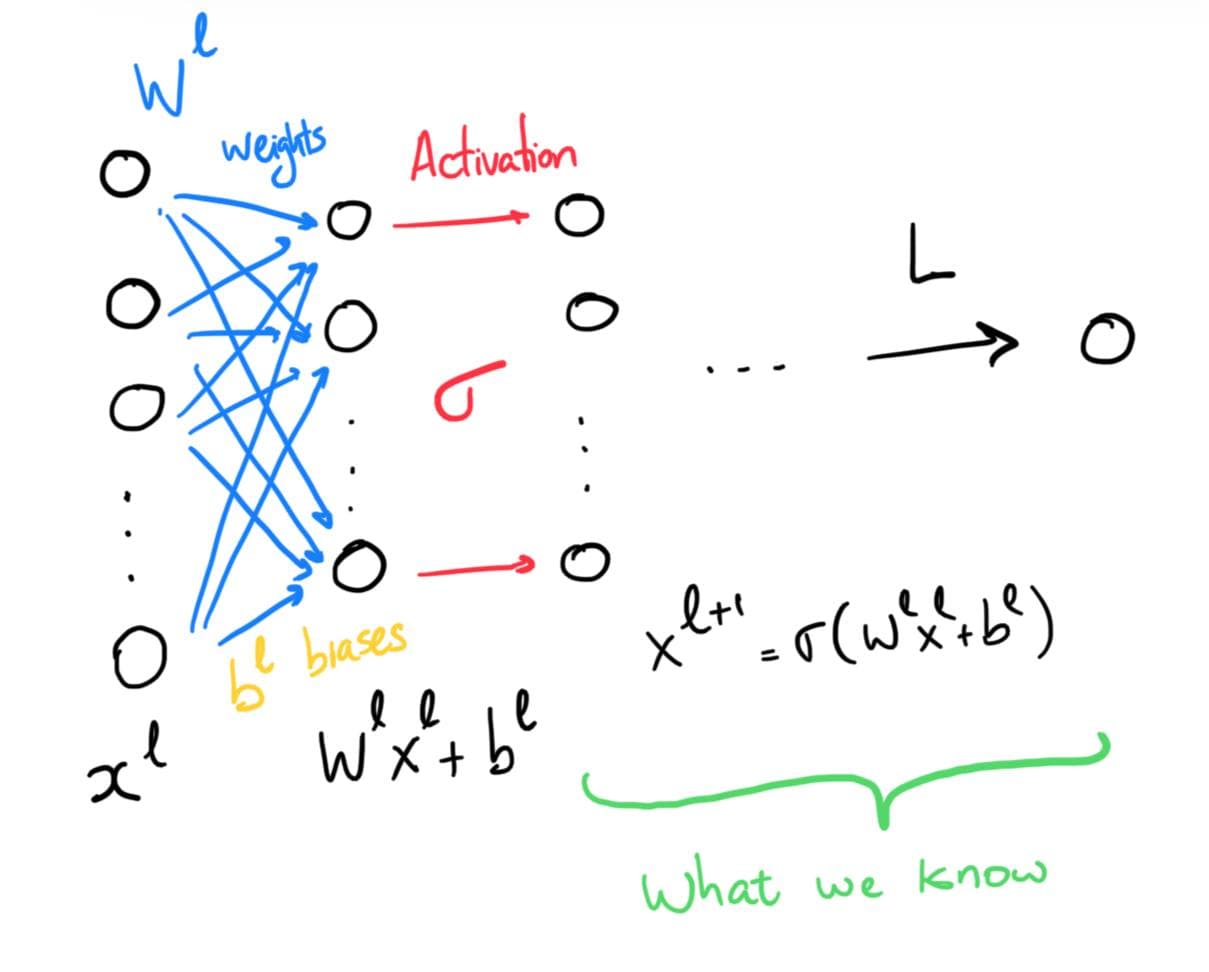
Schematic view of backpropagation.
Suppose that we understand how the loss function changes with respect to the inputs \(\mathbf{x}^{(\ell+1)}\), weights \(W^{(\ell+1)}\) and biases \(b^{(\ell+1)}\) of the \(\ell+1\)-th layer. We would like to use this knowledge to understand how the loss function changes with respect to the inputs, weights and biases of the \(\ell\)-th layer. Mathematically, we can use the chain rule to do this.
Indeed, we can write for each step
$$\dfrac{\partial L}{\partial x^{(\ell)}_i} = \displaystyle\sum_{k} \dfrac{\partial L}{\partial x^{(\ell+1)}_k}\dfrac{\partial x_k^{(\ell+1)}}{\partial x^{(\ell)}_i}.$$
Moreover, the intermediate step is easy to calculate, since \(\dfrac{\partial x_k^{(\ell+1)}}{\partial x^{(\ell)}_i}\) is precisely the derivative of the next layer \(\mathbf{x}^{(\ell+1)} = \sigma(W^{(\ell)}\mathbf{x}^{(\ell)} + b^{(\ell)}).\) More explicitly, the \(k\)-th coordinate is
$$x^{(\ell+1)}_k = \sigma\left(\displaystyle\sum_j W^{(\ell)}_{kj} x^{(\ell)}_j + b^{(\ell)}_k\right),$$
and so the derivative that we’re interested in is
$$\dfrac{\partial x^{(\ell+1)}_k}{\partial x^{(\ell)}_i} = \sigma'\left(\sum_j W^{(\ell)}_{kj} x^{(\ell)}_j + b^{(\ell)}_k\right) W^{(\ell)}_{ki}.$$
It is very useful to write this equation in matrix form. If we denote by \(\nabla_{\mathbf{x}^{(\ell)}}L\) to be the vector with coordinates
$$\nabla_{\mathbf{x}^{(\ell)}}L = \left(\dfrac{\partial L}{\partial x^{(\ell)}_1},\ldots,\dfrac{\partial L}{\partial x^{(\ell)}_n}\right),$$
then the previous discussion tells us that
$$\nabla_{\mathbf{x}^{(\ell)}} L = \sigma'(W^{(\ell)}\mathbf{x}^{(\ell)} + b^{(\ell)}) \odot {W^{(\ell)}}^{\top} \cdot \nabla_{\mathbf{x}^{(\ell+1)}} L$$
where \(\odot\) is the coordinate-wise product between two vectors. Sometimes this is called the Hadamard product.
We can similarly calculate the derivatives with respect to the biases from the equation
$$\dfrac{\partial L}{\partial b^{(\ell)}_i} = \displaystyle\sum_{k} \dfrac{\partial L}{\partial x^{(\ell+1)}_k}\dfrac{\partial x_k^{(\ell+1)}}{\partial b^{(\ell)}_i}.$$
Just like before, we can readily see that
$$\dfrac{\partial L}{\partial b^{(\ell)}_i} = \sigma'\left(\sum_j W^{(\ell)}_{kj} x^{(\ell)}_j + b^{(\ell)}_k\right)$$
and in matrix form this tells us that
$$\nabla_{b^{(\ell)}} L = \sigma'(W^{(\ell)}\mathbf{x}^{(\ell)} + b^{(\ell)}) \odot \nabla_{\mathbf{x}^{(\ell+1)}} L.$$
Again, we can do exactly the same thing for
$$\dfrac{\partial L}{\partial W^{(\ell)}_{ij}} =\displaystyle\sum_{k} \dfrac{\partial L}{\partial x^{(\ell+1)}_k}\dfrac{\partial x_k^{(\ell+1)}}{\partial W^{(\ell)}_{ij}},$$
and also we can calculate
$$\dfrac{\partial L}{\partial W^{(\ell)}_{ij}} = \begin{cases} \sigma'\left(\displaystyle\sum_s W^{(\ell)}_{is} x^{(\ell)}_s + b^{(\ell)}_i\right) x^{(\ell)}_j &\text{ if } k=i \\ 0 &\text{ else.} \end{cases}$$
To deal with the derivative with respect to \(W_{ij}\) in matrix form we can use tensors. The main idea is that instead of thinking of a function in the variables \(W_{ij}\) as \(\mathbb{R}^{n^2}\to\mathbb{R}\) whose gradient is a matrix of size \(n^2\times 1\) we should think of it as a function of \(\mathbb{R}^n\otimes\mathbb{R}^n\to\mathbb{R}\) and so identifying the gradient with a matrix. In simpler terms, we want to think of the gradient as the matrix
$$\nabla_{W^{(\ell)}}L = \begin{pmatrix} \dfrac{\partial L}{\partial W_{11}} & \cdots & \dfrac{\partial L}{\partial W_{1n}} \\ & \ddots & \\ \dfrac{\partial L}{\partial W_{m1}} & \cdots & \dfrac{\partial L}{\partial W_{mn}} \end{pmatrix}.$$
The previous discussion allows us to write this in matrix form as
$$\nabla_{W^{(\ell)}} L = {\mathbf{x}^{(\ell)}}^\top \otimes \left(\sigma'(W^{(\ell)}\mathbf{x}^{(\ell)} + b^{(\ell)})\odot \nabla_{\mathbf{x}^{(\ell+1)}}L\right)$$
where \(\otimes\) is the Kronecker product.
The fundamental thing to realize is that in order to calculate any of the derivatives of \(L\) with respect to the inputs, weights or biases of one layer, we only need the derivative of \(L\) with respect to the inputs of the next layer.
Let us finish this section by recording the relevant equations we have so far
$$\boxed{\nabla_{\mathbf{x}^{(\ell)}} L = \sigma'(W^{(\ell)}\mathbf{x}^{(\ell)} + b^{(\ell)}) \odot {W^{(\ell)}}^{\top} \cdot \nabla_{\mathbf{x}^{(\ell+1)}} L}$$
$$\boxed{\nabla_{b^{(\ell)}} L = \sigma'(W^{(\ell)}\mathbf{x}^{(\ell)} + b^{(\ell)}) \odot \nabla_{\mathbf{x}^{(\ell+1)}} L}$$
$$\boxed{\nabla_{W^{(\ell)}} L = {\mathbf{x}^{(\ell)}}^\top \otimes \left(\sigma'(W^{(\ell)}\mathbf{x}^{(\ell)} + b^{(\ell)})\odot \nabla_{\mathbf{x}^{(\ell+1)}}L\right)}$$
How do we know what loss function to use?
The loss function will depend on each problem, since it’s measuring how far off we are from the right answer. There are two main classes of problems: classification and regression.
In classification problems, we want to predict whether a data point belongs to a certain class. For instance:
- We want to classify an email as spam or not.
- Given morphological data of an Iris flower, we want to distinguish the three species Iris setosa, Iris virginica and Iris versicolor.
- Given a handwritten digit, detect which one from \(0-9\) it is.
In regression problems, we want to predict a certain quantity. For instance:
- We want to predict the price of a house based on certain indicators (size, number of bedrooms, etc.).
- Cost of gas for a certain race circuit.
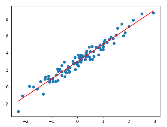
Visualization of a regression problem.
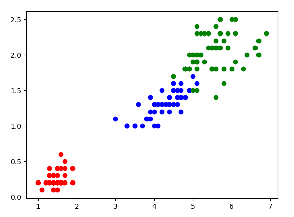
Visualization of a classification problem.
The loss functions will certainly be different, since it’s nothing else but a way of quantifying the error in our predictions. For a classification task we basically want to know how many times we hit the nail and for a regression task we want to know if our prediction was in the right ballpark.
For a regression task, we can use the mean squared error (also known as \(L^2\)-norm). This takes the average of square of the distance between our predictions and the real values. In our previous notation, this is
$$L(\mathbf{y},\widehat{\mathbf{y}}) = \lVert \mathbf{y} - \widehat{\mathbf{y}}\rVert^2=\displaystyle\sum_{i=1}^r ({y}_i-\widehat{y}_i)^2$$
and the total loss is \(\dfrac{1}{M} \displaystyle\sum_{i=1}^M L(\mathbf{y}_i,\widehat{\mathbf{y}}_i).\)
A good thing is that it’s very easy to calculate the derivative of the loss function with respect to \(\mathbf{y}\). Indeed, this is just \(\nabla_{\widehat{\mathbf{y}}} L = -2 (\mathbf{y} - \widehat{\mathbf{y}})\). Remember that this is all we need for the backpropagation!
For a classificatiton task, we can first make it a bit more similar to a regression task by thinking that we want to predict the probability that our data point belongs to each class. In the case that the classification problem has only two labels, this takes the name of logistic regression. Then, to measure the error we can use the cross-entropy, which is a notion of distance between two probability distributions. Despite its esoteric name, in concrete mathematical terms this is just
$$L(\mathbf{p},\mathbf{q}) = - \displaystyle\sum_{\omega\in\Omega}\mathbf{p}(\omega) \log(\mathbf{q}(\omega)) $$
where \(\mathbf{p},\mathbf{q}\) are probability distributions with state space \(\Omega\). Much more concretely, we will think of \(\Omega\) simply as the set \(\{1,\ldots,N\}\) and \(\mathbf{p},\mathbf{q}\) will be vectors in \(\mathbb{R}^N\) whose coordinates add up to \(1\). The \(\log(\mathbf{q}(\omega))\) term allows us to give a larger value to an event of low probability of \(\mathbf{q}\), which is muffled by an event of low probability of \(\mathbf{p}\). Hence if these two probability distributions are similar, they will have the same events of low probability and the cross-entropy will be small.
A very natural way of obtaining a probability distribution is by the use of the softmax function. This is just a higher-dimensional generalization of the logistic function, and is defined as
$$(x_1,\ldots,x_N) \mapsto \left( \dfrac{e^{x_1}}{e^{x_1}+\ldots+e^{x_N}},\ldots,\dfrac{e^{x_N}}{e^{x_1}+\ldots+e^{x_N}} \right).$$
Notice that the coordinates of the vector we obtain add up to \(1\) and so they can be thought of the probability of belonging to each of the classes \(1\) through \(N\). As an aside, notice that if we shift all the numbers by a constant, that is, \(x_1-C,\ldots,x_N-C\), we obtain the same value once we apply the softmax function. This is useful in order to obtain a numerically stable implementation.
It is also useful in this way of thinking to notice that we can think of the vector
$$\mathbf{e}_j=(0,\ldots,\underbrace{1}_{j\text{-th position}},\ldots,0)$$
as encoding the \(j\)-th class, since the probability that it belongs to that class will be \(1\). This takes the name of one-hot encoding. If we think of our training vectors \(\mathbf{y}_i\) as one-hot encodings of the classes, and our predictions \(\widehat{\mathbf{y}}_i\) as applying the softmax function to the result of some layers \(\mathbf{x}_i\), we can write
$$L(\mathbf{y},\mathbf{x}) = -\displaystyle\sum_j y_j \log\left(\dfrac{e^{x_i}}{e^{x_1}+\ldots+e^{x_N}}\right) = \log(e^{x_1}+\ldots+e^{x_N}) - \log(e^{x_k})$$
where \(k\) is the class of \(\mathbf{y}\). Furthermore, it’s easy to see that the derivative with respect to our prediction variable is
\(\nabla_{\mathbf{x}}L = \mathrm{softmax}(\mathbf{x}) - \mathbf{y}\) which is all we need for the backpropagation step.
With this, we have discussed all the math we needed to implement a neural network from scratch!
How do we go about implementing it?
To implement the Linear Algebra operations in C++ we’re going to use the EIGEN library.
We will have an AbstractLayer class. From this class, we will have different layers depending on the activation function \(\sigma\) of our choice. The AbstractLayer class must contain the information of the weights and the biases, and the corresponding gradients with respect to each variable \(W,b\) and \(\mathbf{x}\).
class AbstractLayer {
public:
    // Constructor
    AbstractLayer(int input_size, int output_size) {
        _input_size = input_size;
        _output_size = output_size;
        _weights = 0.1*RandNormalMatrix(output_size,input_size); // Randomly initialize weights
        _biases = VectorXf::Zero(output_size); // Initialize bias as 0
    }

protected:
    int _input_size;
    int _output_size;
    MatrixXf _weights;
    VectorXf _biases;
    MatrixXf _inputs;
    MatrixXf _outputs;
    MatrixXf _gradient_W;
    MatrixXf _gradient_b;
    MatrixXf _gradient_x;
};
Besides the usual setter and getter methods, we need to implement a forwardPass method (that applies the neural network calculation to the input x fixing the weights W and biases b) and backwardPass method (that applies the backpropagation process) and the update step from gradient descent.
    // Calculate output values from inputs, weights and biases
    // For each column vector x in inputs, we do (Wx+b) and then
    // apply the corresponding activation function depending on
    // the kind of layer
    virtual void forwardPass() = 0;
    virtual void backwardPass(const MatrixXf& D) = 0;

    // Stochastic gradient descent allows us to update the weights once
    // we've completed forward and backward pass
    void update(float learning_rate) {
        _weights -= learning_rate*_gradient_W;
        _biases -= learning_rate*_gradient_b;
    }
The usual activation functions that appear on neural networks are Linear, ReLU and Sigmoid. A linear activation function simply takes \(W\mathbf{x}+b\). The ReLU and Sigmoid activation functions are two of the simplest non-linearities we can apply. The ReLU (rectified linear unit) activation function is defined by
$$\mathrm{ReLU}(x) = \begin{cases}x \text{ if }x\geq 0 \\ 0 \text{ else.}\end{cases} $$
More concisely, \(\mathrm{ReLU}(x) = \max(x,0)\). It has the advantage that it is idempotent: this means that no matter how many times we apply the ReLU function, we will get the same result. This is relevant since after many layers the inputs will not get squished, avoiding the problem of vanishing gradients.
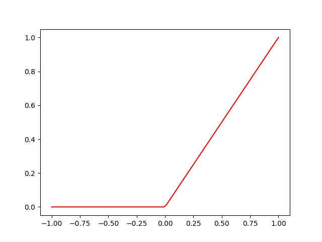
ReLU activation function.
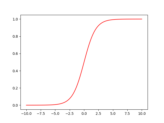
Sigmoid activation function.
The Sigmoid activation function is defined by
$$ S(x) = \dfrac{1}{1 + e^{-x}}.$$
The advantage of the sigmoid function is that it’s smooth and bounded, and it’s derivative is bell-shaped.
Here’s the implementation of the ReLU layer, inheriting from our AbstractLayer class. The implementation of the Linear and Sigmoid layers is very similar.
We only need to calculate the gradient of the pass with respect to each variable. For this we make use of the main equations of the previous section. A word of caution, the actual implementation of this is slightly different because we will want to look at the average of the gradients of a batch instead of a single input vector, but this simplified version contains all of the essential.
// ReLU layer: the activation is the ReLU function
//  =============================================================
class ReLULayer : public AbstractLayer {
public:
    ReLULayer(int input_size, int output_size) : AbstractLayer(input_size, output_size) {}
    void forwardPass() override {
        _outputs = ReLU((_weights*_inputs).colwise() + _biases);
    }
    void backwardPass(const MatrixXf& D) override {
        const MatrixXf z = _weights*_inputs + _biases; // Intermediate step
        _gradient_x = _weights.transpose() * (dReLU_dx(z).asDiagonal()) * D; // .asDiagonal() for the Hadamard product
        _gradient_b =  (dReLU_dx(z).asDiagonal()) * D;
        _gradient_W = KroneckerProduct(_inputs.transpose() , dReLU_dx(z).asDiagonal() * D);
    }
};
We also need a class SequentialLayer to hold all of the layers of the model. This class also has implemented a forwardPass and backwardPass method that activates the corresponding methods in all of the layers (from front to back in the first case and from back to front in the second one).
// Sequential layer: puts together our layers to form the model
//  =============================================================
class SequentialLayer {
public:
    SequentialLayer() {}
    std::vector<AbstractLayer*> getLayers() {
        return _layers;
    }

private:
    std::vector<AbstractLayer*> _layers;
    float _learning_rate;
    MatrixXf _inputs;
    MatrixXf _predictions;
};
Besides the usual setter and getter methods, the forwardPass and backwardPass are implemented as follows
    // Pass the inputs to the first layer and propagate through the entire network
    void forwardPass() {
        _layers[0]->setInputs(_inputs);
        _layers[0]->forwardPass();
        for (std::size_t i = 1; i < _layers.size(); i++) {
            _layers[i]->setInputs(_layers[i-1]->getOutputs());
            _layers[i]->forwardPass();
        }
        // For a classification problem we have to apply softmax to the predictions
        _predictions = _layers[_layers.size()-1]->getOutputs();
    }
    // Do the backward pass starting with D (the differential of the loss)
    // at the last layer, going towards the first layer.
    void backwardPass(const MatrixXf& D) {
        _layers[_layers.siz e()-1]->backwardPass(D);
        _layers[_layers.size()-1]->update(_learning_rate);
        for (int i=_layers.size()-2; i>=0;i--) {
            _layers[i]->backwardPass(_layers[i+1]->getGradient());
            _layers[i]->update(_learning_rate);
        }
    }
Finally, we need our Learner class. This class handles the loss function and the training procedure of the neural network. We need to implement separately the loss functions. We will implement only the mean squared error and the cross-entropy loss functions (so that we can cover both regression and classification problems). Both are straightforward from the discussion on the previous section.
// Calculation of Mean Squared Error function and its derivative:
//  =============================================================
float MeanSquaredError(const MatrixXf& y_pred, const MatrixXf& y_true){
    const int rows = y_pred.rows();
    return (y_true-y_pred).colwise().squaredNorm().sum()/rows;
}

// Derivative of the Mean Squared Error function:
MatrixXf MSEgradient(const MatrixXf& values, const MatrixXf& y_true) {
    const int rows = y_true.rows();
    return (-2*(y_true - values))/rows;
}
// Calculation of Categorical Cross-Entropy loss function and its derivative:
//  =============================================================
float CategoricalCrossEntropy(const MatrixXf& x, const MatrixXf& y_true) {
    const int rows = x.rows();
    MatrixXf y_pred = softmax(x);
    return (y_true.cwiseProduct(log(y_pred))).sum()/rows;
}
// Derivative of the Categorical Cross-Entropy function (composed with softmax)
MatrixXf CCEgradient(const MatrixXf& x, const MatrixXf& y_true) {
    return (softmax(x) -  y_true).rowwise().mean();
}
Now we can implement our training in as many epochs and batches. An epoch is one pass of the entire dataset, and a batch is a group of data that we use to update the weights and biases by taking a step in the average direction of those gradients.
// The learner class allows us to train our model
//  =============================================================
class Learner {
public:
    Learner(const SequentialLayer& model) {
        _model = model;
    }
    // Fit method trains our model
    std::vector<float> fit(const MatrixXf& x_train, const MatrixXf& y_train, int epochs, int batch_size=10, float learning_rate=0.001) {
        _model.setLearningRate(learning_rate);
        _model.setBatchSize(batch_size);
        std::vector<float> losses;
        float loss;
        int iterations;
        for (int epoch=0; epoch<epochs; epoch++) {
            std::cout << "Epoch: " << epoch+1 << std::endl;
            loss = 0.0;
            iterations = 0;
            while (iterations < x_train.cols()/batch_size) {
                std::vector<int> batch(x_train.cols()); // Random subset of size batch_size of samples
                std::iota(batch.begin(),batch.end(),0);
                shuffle(batch.begin(), batch.end(),std::default_random_engine());
                batch.resize(batch_size);
                // Take the columns of x_train and y_train whose indices are in batch
                MatrixXf x_submatrix = MatrixXf::Zero(x_train.rows(),batch_size);
                for (int i = 0; i < batch_size; i++) {
                    for (int j = 0; j < x_train.rows(); j++) {
                        x_submatrix(j,i) = x_train(j,batch[i]);
                    }
                }
                MatrixXf y_submatrix = MatrixXf::Zero(y_train.rows(),batch_size);
                for (int i = 0; i < batch_size; i++) {
                    for (int j = 0; j < y_train.rows(); j++) {
                        y_submatrix(j,i) = y_train(j,batch[i]);
                    }
                }
                loss += fitBatch(x_submatrix,y_submatrix);
                losses.push_back(loss);
                iterations++;
            }
        }
        return losses;
    }

    MatrixXf Predictions(const MatrixXf& input) {
        _model.setInputs(input);
        _model.forwardPass();
        return _model.getPredictions();
    }

private:
    SequentialLayer _model;

    float fitBatch(const MatrixXf& x_train, const MatrixXf& y_train) {
        _model.setInputs(x_train);
        _model.forwardPass();
        // Start with the last gradient for backpropagation
        MatrixXf D = CCEgradient(_model.getPredictions(),y_train);
        _model.backwardPass(D);
        _model.forwardPass();
        return CategoricalCrossEntropy(_model.getPredictions(),y_train);
    }
};
Does it work?
We can use this to build different neural networks with various architectures. We could try the simplest classification toy problem: deciding whether a number is positive or not.
int main() {
    // Artificially created dataset: random numbers labeled positive or negative (one-hot encoding)
    const int samples = 1000;
    MatrixXf x_train = RandNormalMatrix(1,samples);
    MatrixXf y_train = MatrixXf::Zero(2,samples);
    for (int i = 0; i < samples; i++) {
        if (x_train(0,i) > 0) y_train(0,i) = 1;
        else y_train(1,i) = 1;
    }

    // Add layers to our model
    ReLULayer layer(1,2);
    SequentialLayer model;
    model.add(&layer);

    // Train our model
    Learner learner = Learner(model);
    std::vector<float> losses = learner.fit(x_train, y_train, 1000, 100, 0.01);

    // Evaluate our model
    const int test_samples = 100;
    MatrixXf x_test = RandNormalMatrix(1,test_samples);
    MatrixXf y_test = MatrixXf::Zero(2,test_samples);
    for (int i = 0; i < samples; i++) {
        if (x_test(0,i) > 0) y_test(0,i) = 1;
        else y_test(1,i) = 1;
    }
    int count;
    for (int i = 0; i < test_samples; i++) {
        std::cout << "Actual value: " << x_test.col(i) << std::endl;
        std::cout << "Prediction: " << learner.Predictions(x_test.col(i)) << std::endl;
        std::cout << "Predicted value: " << argmax(learner.Predictions(x_test.col(i))) << std::endl;
        if (argmax(learner.Predictions(x_test.col(i))) == argmax(y_test.col(i))) count++;
    }
    std::cout << "Accuracy: " << 100.0*count/test_samples << "%";
    return 0;
}
This shows how to create a simple model, how to add layers, train it and check some simple accuracy metrics. There are still a lot of things to improve: for instance we could use an adaptive optimizer (such as the Adam optimizer) instead of a constant speed variation for each step in our gradient descent. If you are interested, you can find the entire code on my Github page!