Simulating random variables

May 03, 2021

Whenever we are dealing with random events, we would like to have some way to replicate experiments following certain probability distributions. For instance, flipping a (fair) coin is the experiment simulating a Bernoulli random variable of probability $0.5$. However, when we deal with more complicated random variables, it’s not immediately clear how to produce an experiment to simulate them.

Throughout the entire post, we assume that we have some way of generating a (uniform) random number $U$ in $[0,1]$. Our goal is to design experiments to simulate random variables $X$, starting from such $U$. For example, instead of flipping a coin, we could simulate the same outcome by picking a random number $U$ in $[0,1]$ and saying that it’s heads if $U \leq 0.5$ and tails if $U>0.5$.

The “simplest” possible case, is when we know the cumulative distribution function $F(x) = \mathrm{P}(X\leq x)$. In some cases, $F(x)$ is strictly increasing and continuous so it has an inverse function $F^{-1}(p)$, which gives us the unique number $x$ such that $\mathrm{P}(X\leq x) = p$. If we have the knowledge of such an inverse function (sometimes called the quantile function), we can produce a very simple “experiment”.

Inverse transform sampling

Consider a uniform random variable $U$ in $[0,1]$, and suppose that we know the inverse of the cumulative distribution function. Then, to simulate $X$ with the given cumulative distribution function $F$ is as simple as looking at $F^{-1}(U)$.

Indeed, this is because $\mathrm{P}(X\leq x) = \mathrm{P}(F^{-1}(U)\leq x) = \mathrm{P}(U\leq F(x)) = F(x)$. Just notice that the second equality holds because $F$ is an increasing function, and so $a\leq b$ is equivalent to $F(a)\leq F(b)$.

The skeleton of such an implementation in Python is as follows:

import numpy as np

# This is the inverse of the cumulative distribution function of a random variable X we explicitly know
def F_inv(x):
    return #explicit expression

def X():
    U = np.random.uniform(0,1) # Generates a uniform random number between 0 and 1
    return F_inv(U)

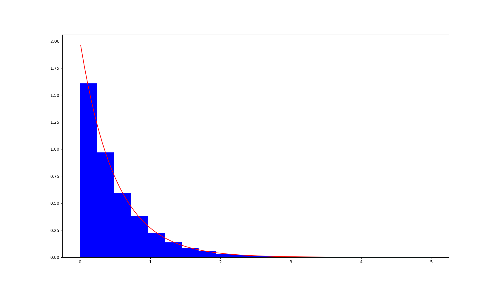
A simple example where we know the inverse of the cumulative distribution function is when $X$ is an exponential random variable. Recall that an exponential random variable $X\sim\mathrm{exp}(\lambda)$ is often used to model the time between events. Its probability density function is given by

$$f_X(x) = \begin{cases} \lambda e^{-\lambda x} &\text{ if } x>0 \\ 0 &\text{ otherwise, }\end{cases}$$

from which we can easily see that the cumulative distribution function is

$$F_X(x) = \displaystyle\int_{-\infty}^x f_X(t)\;\mathrm{d}t = \begin{cases}1-e^{-\lambda x} &\text{ if } x>0 \\ 0 &\text{ otherwise,}\end{cases}$$

and the inverse of the cumulative distribution function is

$$F_X^{-1}(p) = -\dfrac{1}{\lambda}\ln(1-p).$$

Hence we can give a very simple implementation of such a random variable in Python. This is the histogram we obtain after simulating $10000$ rounds of such an experiment (in red, is plotted).

Rejection sampling

The idea of this method is simple. Suppose that we want to sample points in some region. Then we can sample uniformly in a box containing our region and keep (or in scientific terms, accept) the sample if it lies in our region, or reject it if it does not.

For instance, if we want to sample points uniformly in a circle, we may sample points $(x,y)$ in the square $[-1,1]\times[-1,1]$ and accept them if $x^2+y^2 < 1$ or reject them otherwise.

import numpy as np

def sample_circle():
    while True:
        [x,y] = np.random.uniform(-1,1,2)
        if (x**2 + y**2 < 1):
            return [x,y]

The following picture shows $10000$ points generated using this method:

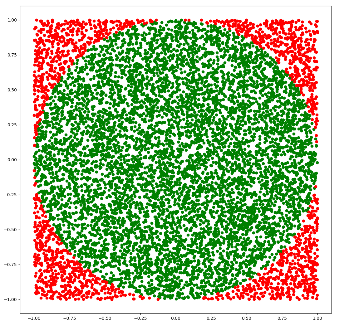Figure: The points in green are the ones we accepted and the points in red are the ones we rejected.

Suppose now that $X$ is a random variable in one dimension. If we plot the probability density function, we can play the same game as above, but with the region below the graph!

This tells us that the method of rejection sampling simulates $X$ from its probability density function $f(x)$.

Now the question is where to sample the points to begin with. We need some sort of envelope, that is, a region that contains our graph from which we will take the points.

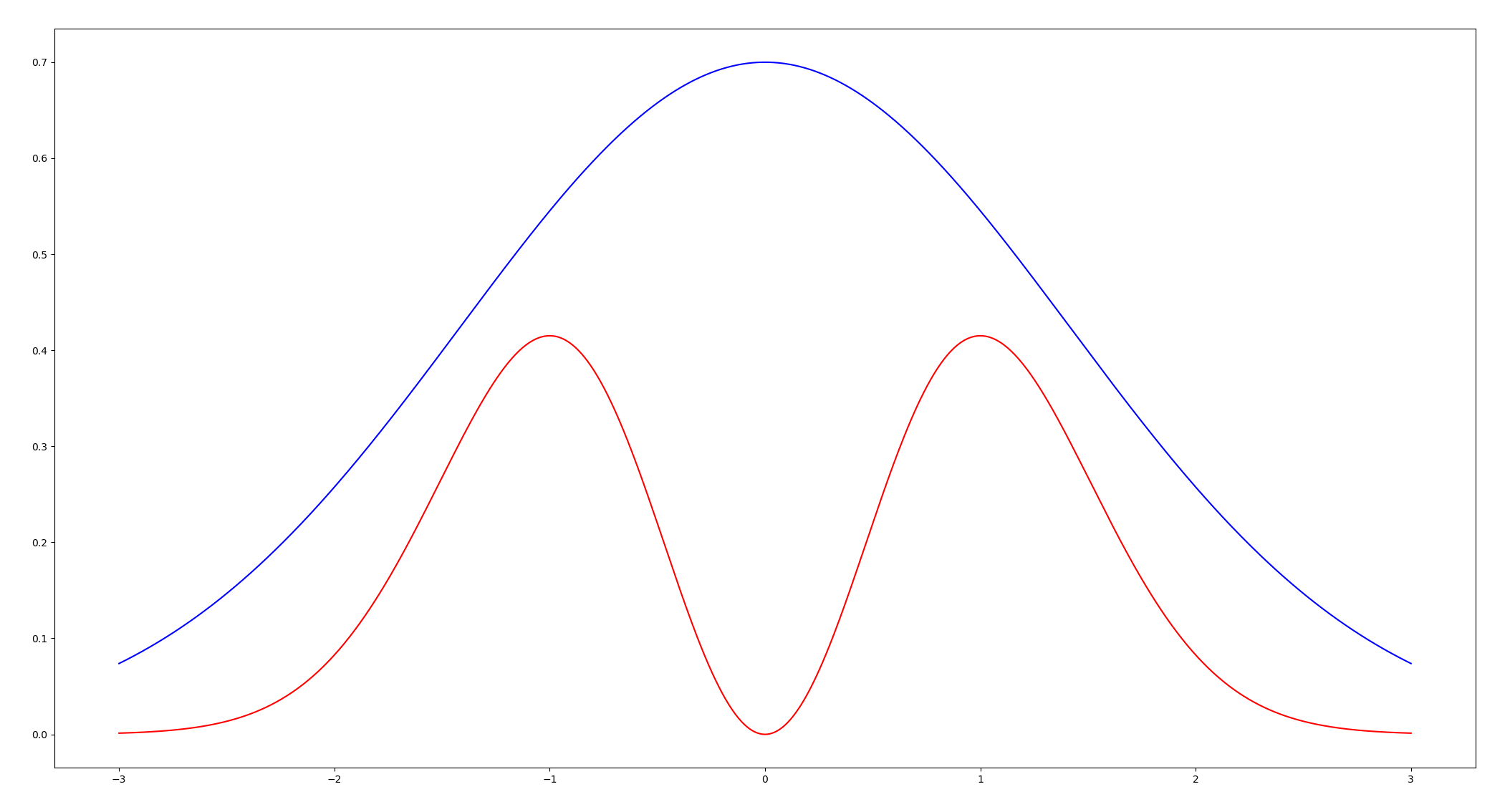Figure: In red, the graph of the probability distribution function we want to simulate, in blue the envelope.

This envelope will generally be the graph of some probability density function $g$ that we know how to simulate, up to some scaling factor $M$.

If we know how to simulate $Y$ with probability density function $g$ such that $Mg(x)\geq f(x)$ for all $x$, then we can simply:

• Simulate from $Y$.
• Generate a uniform random number $U$ in $[0,1]$. (This is independent from the random variable $Y$ we generated in the previous step).
• We accept the sample if $U < \dfrac{f(Y)}{Mg(Y)}.$
• We reject it otherwise and take a new sample.

The skeleton of the code will look something like this:

import numpy as np

def f(x):
    return # explicit expression

def g(x):
    return # explicit expression

def simulate_Y():
    return # explicit method to simulate random variable with pdf g

def rejection_sampling():
    while True:
        U = np.random.uniform(0,1)
        Y = simulate_Y()
        if U < f(Y)/(M*g(Y)):
            return Y

Rejection sampling for a Normal variable

As an example, let’s show how to simulate a normal distribution $X\sim N(0,1)$ with zero mean and standard deviation $1$.

The first observation is that, by symmetry, it’s enough to sample from the absolute value $\vert X\vert$. Indeed, if we know $\vert X\vert$ then we just generate a sign $S=\pm 1$ with probability $0.5$ and set $X = S\vert X\vert$.

The density function of $\vert X\vert$ is given by

$$f(x) = \dfrac{2}{\sqrt{2\pi}} e^{-x^2/2}, \;\;x\geq 0.$$

As an envelope, we can take the exponential distribution $g(x)=e^{-x}$ (which we know how to simulate by the previous example!).

The scaling factor $M$ is given by the maximum value of $\dfrac{f(x)}{g(x)} = e^{x-x^2/2} \sqrt{2/\pi}$, which occurs at $x=1$. We get, in that case, that $\dfrac{f(x)}{Mg(x)} = e^{-(x-1)^2/2}.$

import numpy as np

def f(x):
    return 2*np.exp(-x**2/2)/np.sqrt(2*np.pi) if x>= 0 else 0

def g(x):
    return np.exp(-x) if x>=0 else 0

def simulate_Y():
    U = np.random.uniform(0,1)
    return -np.log(U)

def rejection_sampling():
    while True:
        U = np.random.uniform(0,1)
        Y = simulate_Y()
        if U <= np.exp(-(Y-1)**2 / 2):
            S = 1 if np.random.uniform(0,1)>0.5 else -1
            return S*Y

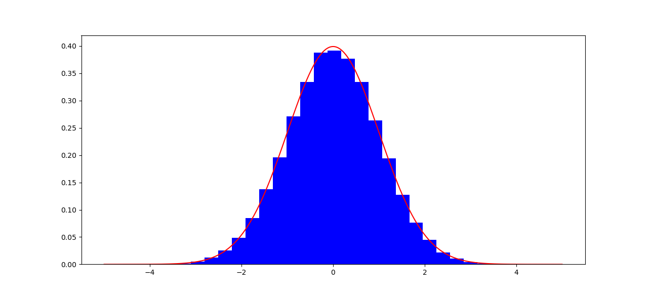
Below we can picture the histogram of $100000$ points generated using this algorithm, together with the actual density function in red.

In the next post, we will see some more sophisticated sampling techniques, such as Markov Chain Montecarlo methods, the Metropolis-Hastings algorithm and Gibbs sampling.

You can find all the code involved in this post on my GitHub.