In a previous post, we discussed different methods to simulate probability distributions. In this post, we are going to explain how to simulate discrete probability distributions in essentially \(O(1)\) time (after some preprocessing).
The idea
Our goal is to simulate efficiently a random variable taking values \(\{a_1,\ldots,a_n\}\) with probability \(\{p_1,\ldots,p_n\}\) respectively.
This is a familiar problem in simpler cases: if we flip a coin, we’re just getting a random variable with values \(\{\mathrm{Heads},\mathrm{Tails}\}\) each with probability \(0.5\). To do that, we can simply draw a uniform random number \(U\in(0,1)\) and claim that it’s \(\mathrm{Heads}\) if \(U\leq 0.5\) and \(\mathrm{Tails}\) otherwise.
The underlying geometric idea is the same as we used when talking about the rejection sampling method: If we throw a dart to a dartboard, the probability that it lands inside of a given region is the area of the region divided by the total area of the dartboard.
We can think of our situation by having rectangles of width \(1\) and height \(p_i\). The problem is that if we bound our rectangles into a larger rectangle, every time we choose a point that is not in any of our rectangles, we would have to choose a new point. This is just as we discussed with rejection sampling.
Think of the case where we have four possible outcomes with probabilities \(0.60, 0.25, 0.10\) and \(0.05\). If we stack the rectangles then there’s still a lot of gray space as in the picture.

However, if we could cleverly slice up our rectangles and fit them together into a single rectangle in a Mondrianesque picture, we wouldn’t have that problem.

That’s what the Alias Method does!
The Alias Method
Now that we understand the idea, we can describe how to associate the alias to each region. This is the preprocessing step that will allow us to simulate the given distribution in \(O(1)\) time.
We follow the implementation in Vose’s article “A linear algorithm for generating random numbhers with a given distribution”.
Vose uses two tables for the preprocessing: a prob table and an alias table. The first one keeps track of the heights of the rectangles as we’re slicing them around and the second one keeps track of their positions.
import numpy as np
class AliasMethod:
    def __init__(self, dist):
        self.dist = dist
        self.createAlias() # Initializes the prob and alias tables
First, we divide the indices in two groups large and small: an index \(j\) is large if \(p_j > \frac{1}{n}\) and small otherwise. We want to break up the excedent in those rectangles for the large indices, and take it into the small indices. To do that, we take the excedent \(p_j-\frac{1}{n}\) and move it to the corresponding pile (the alias).
We initialize the prob table by scaling the probability distribution dist we’re given by the number of possible states \(n\). We think of dist as a dictionary \(\{a_i : p_i \text{ for }i\in \mathrm{range}(n) \}\) whose keys are the possible states and the values are the corresponding probabilities.
def createAlias(self):
    n = len(self.dist)
    self.prob = {}
    self.alias = {}

    small, large = [], []
    for x in self.dist:
        self.prob[x] = n * self.dist[x]
        if self.prob[x] < 1:
            small.append(x)
        else:
            large.append(x)
We’re in conditions of creating the alias table.
while small and large:
    s = small.pop()
    l = large.pop()

    self.alias[s] = l

    self.prob[l] = (self.prob[l] + self.prob[s]) - 1

    if self.prob[l] < 1:
        small.append(l)
    else:
        large.append(l)

while large:
    self.prob[large.pop()] = 1
while small:
    self.prob[small.pop()] = 1
Notice that this procedure is clearly \(O(n)\) in time complexity. Indeed, the classification of indices as small or large only looks at each label once, and then we decrease the number len(small)+len(large) (which starts being \(n\)) in each step.
We can generate a random sample now by choosing one of the \(n\) rectangles uniformly, choosing a uniform random number in \((0,1)\) and returning the index of the rectangle if we’re below the prob threshold or the corresponding alias otherwise.
def generateRandom(self):
    rect = np.random.choice(list(self.dist.keys()))
    if self.prob[rect] >= np.random.uniform():
        return rect
    else:
        return self.alias[rect]
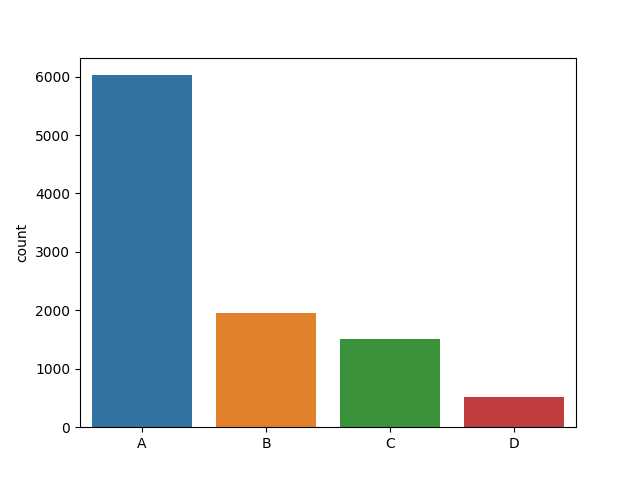
And that’s it! We can now put it to the test with dist = {'A':0.6,'B':0.20,'C':0.15,'D':0.05} as in the example. The following plot shows how many samples of each kind we obtain as we sample \(10000\) times using this method. As we can see, in this “experiment”, \(A\) appears \(6024\) times, \(B\) appears \(1955\) times, \(C\) appears \(1506\) times, and \(D\) appears \(515\) times.

You can find this implementation of the Alias method on my Github.